First Order Equations
We start off easy with four examples of first order equations:
\frac{dy}{dt} = y \tag{1}
\frac{dy}{dt} = -y \tag{2}
\frac{dy}{dt} = 2ty \tag{3}
\frac{dy}{dt}=y^2 \tag{4}
Equations Equation 1, Equation 2, and Equation 3 demonstrate linear differential equations; Equation 4 is nonlinear. Equation 3 has a variable coefficient term; the other linear equations are linear constant coefficient.
Each equation has a family of solutions (particular solution + null solutions). The null solutions will contain a +C term determined by the value of y(0). Here is the solution to the simplest differential equation of all:
\frac{dy}{dt} = f(t) \hspace{1em} \textnormal{The solution is:} \hspace{1em} y(t) = \int_0^t f(s)\,ds + C
Here are the solutions to our simple equations:
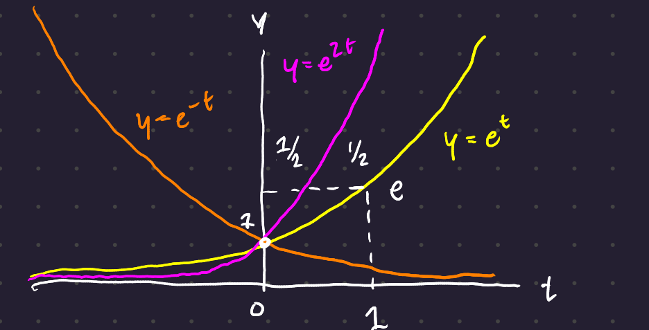
Equation 1 is solved by y(t) = e^t
Equation 2 is solved by y(t) = e^{-t}
Equation 3 is solved by y(t) = e^{t^2}
Equation 4 is solved by y(t) = \frac{1}{1-t}
The linear equations are solved by powers of e; the nonlinear diffeq is solved by a different type of function. \frac{dy}{dt}\left(\frac{1}{1-t}\right) = \frac{1}{(1-t)^2}
Our final example extends Equation 1 and Equation 2 to allow any coefficient a:
\frac{dy}{dt} = ay \hspace{3em} y(t) = Ce^{at}
1 Short Calculus Refresher
1.1 Derivatives of Key Functions
Here are the derivatives (and derivations) for several key functions:
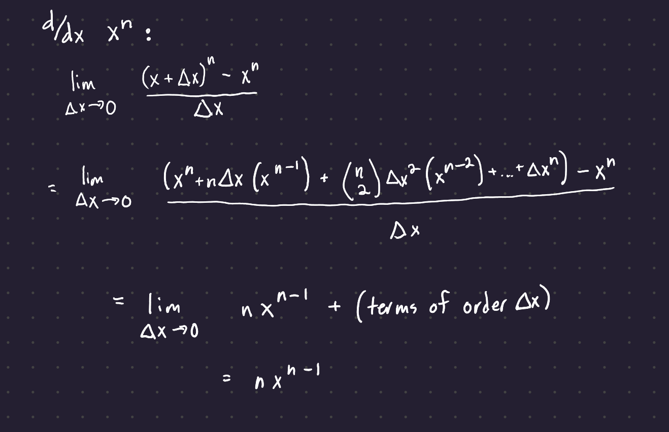
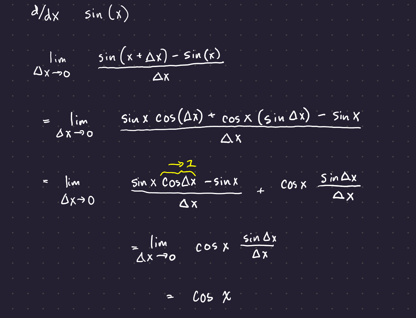
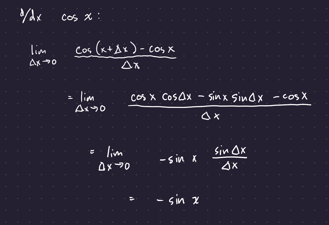
The derivative of e^x is its most useful property, and the proof of its derivative differs based on how you derive your formula for e^x. The derivative of of ln(x) comes from properties of logarithms: is a complete mystery.
1.2 Rules for Derivatives:
1.2.1 Sum Rule:
The derivative of the sum of two functions is the sum of the derivatives:
\frac{d}{dt}(f + g) = \frac{df}{dt} + \frac{dg}{dt}
This is important - the derivative operator is a linear transformation.
1.2.2 Chain Rule:
This allows you to find the derivatives of most composite functions. If y = e^x and x = \sin t,
\frac{dy}{dt} = \frac{dy}{dx}\frac{dx}{dt} = e^x\cos t = y\,\cos t
The product rule and quotient rule are simply applications of the chain rule to the functions y = fg and y = f/g.
1.3 Fundamental Theorem of Calculus
The derivative of the integral of f(x) is f(x). \int_0^x \frac{df}{dx}dx = f(x) - f(0)
This can be remembered as a sum of differences:
(y_1 - y_0) + (y_2 - y_1) + ... + (y_n - y_{n-1}) = y_n - y_0
To make this into an integral of a derivative, each difference term is divided by \Delta x, and then the result is multiplied by \Delta x, creating no total change.
More importantly,
\frac{d}{dx}\int_a^x f(s)\,ds = f(x)
The sum of difference can be thought of equivalently as a sum of differences or as a difference of sums.
1.4 Derivatives as Slope Approximations
You can use a derivative to create a linear approximation of a function around a point.
\Delta y \approx \Delta x\,\frac{dy}{dx}
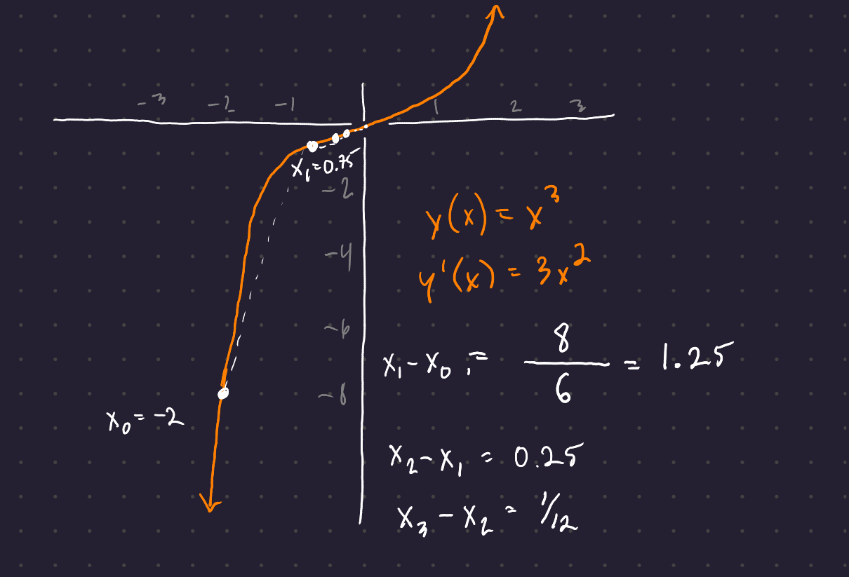
We can also derive Netwonn’s methodd to solve y(x) = 0 starting at x(0). \Delta x \approx \Delta y / \frac{dy}{dx} \hspace{2em} x_1 - x_0 = \frac{-y(x_0)}{dy/dx\,(x_0)}
You know how much you want to change (you want to go from y=y(x_0) to y=0, and you know the slope of the function at the current point. Newton’s method lets you get there.)
2 Taylor series
Our linear approximation is improved when we make it a second-order polynomial that permits bending of the graph:
y(x_0 + \Delta x) \approx y_0 + (\Delta x)y'_0 + 1/2(\Delta x)^2 y''_0
Adding (\Delta x)^2 takes us from constant slope to constant bending (quadratic approximation). We can improve our performance in the limit by simply adding infinitely many terms:
y(x_0 + \Delta x) = \sum_{n=0}^{\infty} \frac{(\Delta x)^n}{n!}y^{(n)}(x_0)
This equation only applies if the equation is both continuous beyond x_0, and if every derivative of the function remains continuous after x_0. These properties are satisfied for most basic functions, but may not be satisfied for more realistic ones (and definitely aren’t satisfied for steps, ramps, and delta functions.)
We can get Taylor series for our favorite functions. First is the exponential series with y^{(n)}(0) = 1:
y = e^x = 1 + x + \frac{1}{2!}x^2+ \frac{1}{3!}x^3+ \frac{1}{3!}x^3 + ...
Next is the geometric series with y^{(n)} x_0 = n!:
y = \frac{1}{1-x} = 1 + x + x^2+ x^3+ x^4 + ...
3 Application to y’ = ay + q(t)
This is important enough to get its own section.
y' = a\,y + q(t) is a perfect multipurpose model, with growth rate a and external source (forcing) term q(t).
\frac{dy}{dt} = ay + q(t) \hspace{1em} \textnormal{is solved by} \hspace{1em} y(t) = \int_0^t e^{a(t-s)}\,q(s)\,ds
At each time s between 0 and t, the input is a source of strength q(s). That input grows or decays over the remaining time t-s. e^{a(t-s)} times q(s) gives the result of the growth of that input at time t. We then integrate over all times s between 0 and t to find the total growth of the input function q(t).
4 Four Particular Solutions
Key ideas: 1. The complete solution to a linear equation is the null solution(s) + the particular solution. 2. The integrating factor e^{-at} multiplies y' - ay = q(t) to give our general solution for any input q(t): $y(t) = e^{at},y(0) + e^{at}_0^t ,e^{-as},q(s),ds 3. For y' - ay = q = constant, the very particular solution is q(e^{at} - 1)/a 4. q(t) = H(t): the response to a unit step function is y_p = (e^{at} - 1)/a 5. q(t) = \delta(t): the response to a unit delta function is y_p = e^{at} 6. q(t) = e^{ct} gives y_p = (e^{ct} - e^{at})/(c-a). In case c = a, change to y_p = t\,e^{at}.
We start with dy/dt = ay, which is solved by y(t) = e^{at}\,y(0).
Now we look at 4 particularly important inputs q(t) and responses y(t):
- Constant source q(t) = q
- Step function at T q(t) = H(t-T)
- Delta function at T q(t) = \delta(t-T)
- Exponential input q(t) = e^{ct}
4.1 Solving Linear Equations with an Integrating Factor
We choose an integrating factor M(t) such that M (y' - ay) = \frac{d}{dt}(My).
The factor is chosen by the chain rule: \begin{align} \frac{d}{dt}(My) &= y\frac{dM}{dt} + M\frac{dy}{dt} \\ M (y' - ay) &= y \, M' + M \, y' \\ -M\,a\,y &= y\,M' \\ -M\,a &= M' \\ M &= e^{-at} \end{align}
After multiplication by M, you can integrate both sides from 0 to t:
\begin{align} \frac{d}{dt}(My) &= Mq \\ M(t)\,y(t) - M(0)\,y(0) &= \int_0^t M(s)\,q(s)\,ds \\ y(t) &= \frac{y(0)}{M(t)} + \frac{1}{M(t)}\int_0^t M(s)\,q(s)\,ds \\ y(t) &= e^{at}y(0) + e^{at}\int_0^t e^{-as}\,q(s)\,ds \end{align} \tag{5}
This strategy of finding an integrating term M will return when our equations stop being linear.
4.2 Constant source q(t) = q
A constant source creates a pretty easy integration:
\int_0^t e^{-as}\,q\,ds = \left[ \frac{qe^{-as}}{-a}\right]_{s=0}^{s=t} = \frac{q}{a}(1 - e^{-at})
(keep an eye on the signs!)
The full solution (right side divided by M(t) = e^{-at} is then
y(t) = e^{at}\,y(0) + \frac{q}{a}(e^{at} - 1)
When a is negative, the equation approaches a steady state -q/a. Here the derivative y' = ay + q is zero, so no change can occur.
4.3 Heaviside Step Function
H(t) jumps from 0 to 1 at t=0. Its shift H(t-T) jumps to 1 at t=T.
When the step comes at t=0, the solution to y' - ay = H(t) is the step response (scaled exponential curve shifted downwards by 1/a). The starting value y(0) = 0, and all values to the left of 0 are 0.
y(t) = \frac{1}{a}(e^{at} - 1)
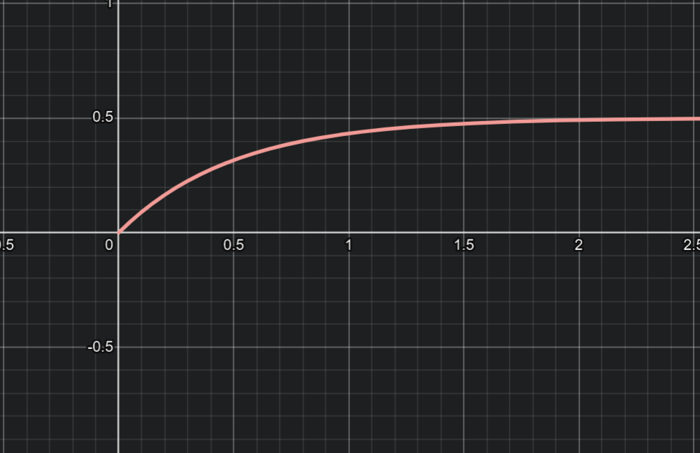
When the heaviside step kicks in at t=T instead of t = 0, you add in the step response beyond that time T (the integral on the right side is \int_T^te^{-as}\,ds).
y(t) = \left\{ \hspace{0.5em} \begin{matrix} y(0) e^{at},& t < T \\ y(0)e^{at} + \frac{1}{a}(e^{at} - 1),& t > T \end{matrix} \right.
4.4 Delta Function
Oh hey, it’s Strang’s favorite “illegal” function, \delta(t).
The “delta function” is everywhere 0, except for at t=0, where it gives a unit input. Here are a few ways to think about \delta(t):
- As a point source concentrated at t=0. If you take the integral of the delta function between -\Delta x and \Delta x, the integral is always 1, even as \lim_{\Delta x \to 0}.
- As the derivative of the Heaviside function H(t). The Heaviside function has no slope except for at t=0, where it suddenly jumps up by one.
Step functions are best understood by their integrals:
\begin{align} \int_{-\infty}^{\infty} \delta(t) \, dt &= 1 \\ \int_{-\infty}^{\infty} \delta(t) \, F(t) dt &= F(0) \\ \int_{-\infty}^{\infty} \delta(t-T) \, F(t) dt &= F(t) \end{align}
Since the delta function is the derivative of the step function, the impulse response must be the derivative of the step response:
\frac{d}{dt}(\texttt{Step Response}) = \frac{d}{dt}\left(\frac{e^{at} - 1}{a}\right) = e^{at} = \texttt{Impulse Response}
The impulse response y(t) jumps immediately to y(0)=1:
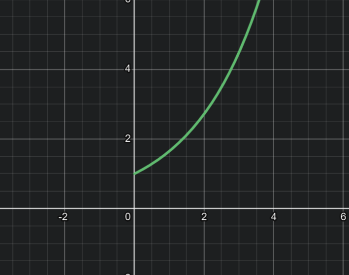
Key realization: e^{at} is the growth factor G(t) for all inputs. Since our input is an instantaneous input of 1 at time 0, the impulse response is simply the growth factor distilled into its purest form. This is what the delta function lets us see!
If you delay the delta function, you add the growth term only after the time of the impulse:
y(t) = e^{at} \, y(0) + e^{a(t-T)} \hspace{0.5em} \textnormal{for}\hspace{0.5em}t>T.
4.5 Exponential Input
Exponential input would describe growth, decay, or oscillation.
The particular solution to an exponential source e^{ct} is simply a multiple Ye^{ct} of the same exponential function. Simply substitute Ye^{ct} into y' - ay = e^{ct}:
cYe^{ct} - aYe^{ct} = e^{ct}
Then cancel out e^{ct} (never equal to zero):
\begin{gather} cY - aY = 1 \\ Y = \frac{1}{c-a} \\ y_p(t) = \frac{e^{ct}}{c-a} \end{gather}
This particular solution is alright, but it doesn’t equal 0 at t=0, which makes it a little less nice to work with. We can fix it by adding to the null solution:
y_{\textnormal{complete}} = y(0)e^{at} - \frac{e^{at}}{c-a} + \frac{e^{ct}}{c-a}
4.5.1 Resonance
When c = a there is trouble: the denominator 1/(c-a) does not exist. We go back to the mainn formula Equation 5 to figure out our solution:
y' - ay = e^{at} \hspace{1em} \textnormal{means} \hspace{1em} y = y(0)e^{at} + e^{at}\int_0^t e^{-as}\,e^{as}\,ds
The integral evaluates to \int 1\, ds = t:
y = y(0)e^{at} + t\,e^{at}
5 Real and Complex Sinusoids
Split into its own document, see the link here