Structural Mechanics Coursework
1 Load and Stress in a Truss
1.1 Setup
In this section, data from strain gauges is analyzed to determine the force applied to a truss structure.
The truss structure is shown in Figure 1.1.
Figure 1.2 labels the internal forces evolved when a force f is applied to point E in the truss.
By summing the forces at each point to 0, the following relationships are obtained:
| Force | Amount | Sense |
|---|---|---|
| f_1 | \sqrt{2}f | Tension |
| f_2 | f | Compression |
| f_3 | f | Compression |
| f_4 | f | Tension |
| f_5 | \sqrt{2}f | Tension |
| f_6 | 2f | Compression |
These forces create stress within the trusses
\sigma = \frac{F}{A}, \tag{1}
where A = 250~\mathrm{mm}^2 is the cross-sectional area of the truss.
The strain associated with a stress \sigma is
\epsilon = \frac{\sigma}{E}, \tag{2}
where E = 2.5~\mathrm{GPa} is the Young’s modulus of acrylic.
1.2 Results
The strain values are shown in Table 2, and the relationship between strain and slider position is graphed in Figure 1.
| Slider | Gauge 1/\mu \epsilon | Gauge 2/\mu \epsilon | Gauge 3/\mu \epsilon | Gauge 4/\mu \epsilon | Gauge 5/\mu \epsilon | Gauge 6/\mu \epsilon |
|---|---|---|---|---|---|---|
| 0 | -1.1 | -0.01 | 0.3 | 1.21 | 0.46 | -0.91 |
| 3 | 0.23 | 0.04 | 1.01 | 0.16 | 0.4 | 1.83 |
| 6 | 23.2 | -17.51 | -15.91 | 16.74 | 23 | -34.32 |
| 9 | 101.36 | -76.16 | -77.43 | 67.6 | 101.42 | -156.98 |
| 12 | 197.83 | -151.34 | -155.06 | 128.08 | 197.53 | -310.97 |
| 15 | 314.3 | -235.97 | -249.47 | 198.57 | 305.93 | -482.21 |
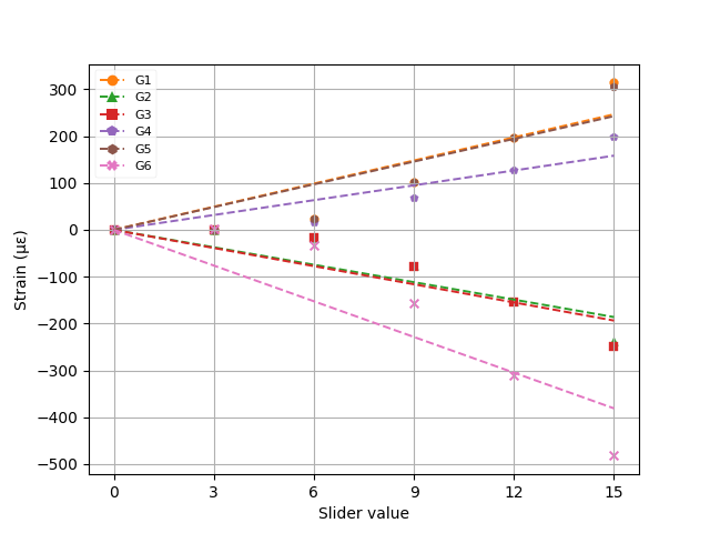
The slope of the line of best fit, as well as the R^2 coefficient for each line, is given in Table 3.
| Gauge | Slope | R^2 | Force/ N |
|---|---|---|---|
| G1 | 16.44 | 0.90 | 10.28 |
| G2 | -12.41 | 0.90 | -7.75 |
| G3 | -12.91 | 0.89 | -8.06 |
| G4 | 10.55 | 0.91 | 6.59 |
| G5 | 16.18 | 0.90 | 10.11 |
| G6 | -25.41 | 0.90 | -15.88 |
According to this analysis, one tick on the slider would correspond to an applied force of 7.45~\mathrm N with a standard deviation of 0.51 N.
1.3 Discussion
Two distinct sources of error were identified. First is the unavoidable random error created by imprecision in measuring the strain gauges. Over the course of the experiment, the strain gauges were observed to vary by \pm 5 ~\mu \epsilon. The second and much more significant source of error is backlash in the force-applying mechanism. No increase in strain was observed between slider values of 0 and 3. This suggests that the mechanism did not begin to apply force to the truss until at least a slider value of 3. Such backlash is normally avoided by applying preload to a mechanism; it’s likely that if the zero value on the slider corresponded to a non-zero amount of applied force, such backlash would not be observed.
1.4 Postscript
To see the effect of the systematic error caused by backlash, the linear regression was repeated starting at a slider value of 3 instead of the slider value of 0. The results from this analysis are given in Table 4 and Figure 2.
| Gauge | Slope | R^2 | Force/ N |
|---|---|---|---|
| G1 | 23.07 | 0.97 | 14.41 |
| G2 | -17.41 | 0.97 | -10.88 |
| G3 | -18.15 | 0.96 | -11.34 |
| G4 | 14.78 | 0.97 | 9.24 |
| G5 | 22.69 | 0.97 | 14.18 |
| G6 | -35.66 | 0.97 | -22.29 |
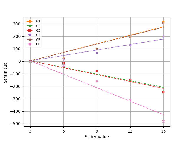
In this analysis, one tick on the slider would correspond to an applied force of 10.47~\mathrm N with a standard deviation of 0.73 N.
It is worth noting that, although removing the first measurement increased the accuracy of the linear regression (as indicated by the increased R^2 values), it increased the deviation in the force estimate. Also, from examining Figure 2, it still appears that the strain does not increase linearly with slider value. Further investigation could reveal the source of this non-linear error.
2 Composite Action in a Beam
2.1 Setup
In this section, beams of composite construction are loaded, and the evoked internal strains are compared against predictions from Euler beam theory.
The force F applied to the beam is created by the following lever system:
A simple moment analysis indicates that
F = \frac{n}{m}W \tag{3}
This force F is applied equally at two point loads midway along the beam, with the strain gauge placed at point P.
The internal moment M generated at point P can be found by a simple free-body diagram:
Summing the moments about P to zero, we find that
M = 425~\frac{F}{2} = 212.5~F \tag{4}
To find the behavior of the beam under this moment, we create an equivalent, all-steel beam with a lower width of
b_{s} = b_a~\frac{E_a}{E_s}= 30~\frac{7}{20}
The centroid of this beam is located 18.12 mm from the top of the beam, and it has a second moment of area I_{eff} of 98718 mm^4.
For a given moment M, we calculate the curvature
\kappa = \frac{M}{EI},
which we can use to find the strain at a height y
\epsilon = \kappa y.
These relationships hold because the load on the beam is incident on a principal axis of the beam.
2.2 Results
| Weight/ N | Gauge 1/ \mu \epsilon | Gauge 2/ \mu \epsilon | Gauge 3/ \mu \epsilon | Gauge 4/ \mu \epsilon | Gauge 5/ \mu \epsilon | Gauge 6/ \mu \epsilon |
|---|---|---|---|---|---|---|
| 30 | -13.3648 | 17.6874 | -100.6451 | 12.6810 | 5.61706 | 100.6510 |
| 60 | -31.3564 | 41.3451 | -204.0247 | 24.5087 | 10.6981 | 204.6510 |
| 90 | -49.6545 | 63.0456 | -309.5608 | 36.1560 | 14.1569 | 309.4564 |
| 120 | -68.3243 | 88.0254 | -417.6570 | 49.1061 | 21.6059 | 416.4505 |
| 150 | -87.6473 | 113.025 | -526.6406 | 60.5640 | 26.1606 | 525.2050 |
| Weight/ N | Gauge 1/\mu \epsilon | Gauge 2/\mu \epsilon | Gauge 3/ \mu \epsilon | Gauge 4/\mu \epsilon | Gauge 5/\mu \epsilon | Gauge 6/\mu \epsilon |
|---|---|---|---|---|---|---|
| 30 | -46.6051 | -34.6504 | -33.6051 | 19.3210 | 19.2610 | 65.2601 |
| 60 | -96.5406 | -70.0546 | -70.5061 | 41.2510 | 40.6210 | 136.510 |
| 90 | -150.106 | -109.561 | -109.061 | 63.6510 | 62.2610 | 211.610 |
| 120 | -206.514 | -150.501 | -149.006 | 88.6501 | 85.6901 | 289.261 |
| 150 | -251.650 | -182.561 | -182.652 | 107.212 | 103.650 | 352.620 |
2.3 Discussion
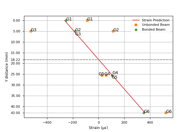
From Figure 3, the internally bonded beam had internal strains closely matching the prediction from Euler beam theory. However, the beam without the internal bond varied significantly from the predicted stress, with large discrepancies over the entire cross-section.
The discrepancy between prediction and experiment for the unbonded beam stems from the fact that Euler beam theory requires planar sections within the beam to remain planar. In the bonded beam, plane sections across the transition must remain planar, but the unbonded beams were able to shift relative to each other.
The result of this shift is that the unbonded case acts like two independent beams: the measured strain at Gauge 2 (the bottom of the steel section) is actually positive, indicating that the bottom of the steel section is in tension, instead of the expected compression. Contrast this with the bonded beam, where Gauge 2 and Gauge 3 (measuring the strain in the bottom of the steel section and the top of the aluminum section, respectively) have the same negative strain.
3 Torsion of a Shaft
3.1 Setup
In this section, a torque is applied to shafts of different materials via a lever arm, and the deflection of the lever arm is measured.
The experimental setup is illustrated in Figure 3.1:
The weight W acting on a lever arm creates a torque T in the shaft:
The torque on the shaft is
T = 100~W
This torque causes the beam to twist, which creates a deflection in the lever arm. This deflection is measured by a dial indicator at point P.
The distance \delta_l between P and \mathrm P' gives the angle of twist \phi of the bars:
\sin\phi = \frac{\delta_l}{55} \tag{5}
Since \phi is small, we can apply the fundamental theorem of engineering
\sin\phi \approx \phi \tag{6}
and thus (by Equation 5)
\phi = \frac{\delta_l}{55} \tag{7}
The general expression for torsion in a uniform member is given by
\phi = \frac{TL}{GJ} \tag{8}
where L = 280~\mathrm{mm} is the length of the bar and J is the torsion constant of the bar. For a bar 10mm in diameter,
J = \frac{\pi r^4}{2} = 981.7~\mathrm{mm^4} \tag{9}
First the deflection of the equipment is measured with no twist in the bar. The mechanism is expected to flex slightly under load without the beam twisting, and this flexure must be subtracted from the subsequent measurements. Then the deflections are measured for steel and aluminum bars; for each test, the lever arm is loaded with 0.9kg and 1.8kg weights.
3.2 Results
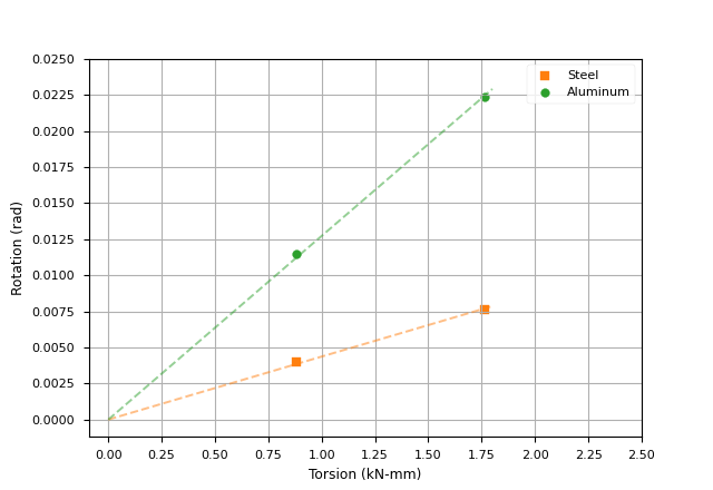
| Material | Mass/ kg | Deflection/ mm | Corrected Deflection/ mm | Torque/ kN-mm | Rotation/ rad |
|---|---|---|---|---|---|
| Steel | 0.9 | 0.30 | 0.22 | 0.88 | 0.0040 |
| Steel | 1.8 | 0.58 | 0.42 | 1.77 | 0.0076 |
| Aluminum | 0.9 | 0.71 | 0.63 | 0.88 | 0.012 |
| Aluminum | 1.8 | 1.39 | 1.23 | 1.77 | 0.022 |
Using the experimental results and Equation 8, the shear moduli of steel and aluminum were calculated.
| Material | Shear Modulus G/ \mathrm{kN/mm^2} |
|---|---|
| Steel | 64.5 \pm 1.5 |
| Aluminum | 22.3 \pm 0.3 |
3.3 Discussion
The most likely source of error in the estimates is in the measurements from the dial indicator. Although the indicator is precise and accurate, it is difficult to obtain repeatable sub-millimeter precision over the course of an experiment. If the tip of the dial indicator drifted slightly over the course of loading and unloading the beam, or the support structure shifted by a few hundredths of a millimeter, it would introduce a systematic error to all measurements made after the shift. This error can be minimized by the experimenter, but it takes extreme care and caution to obtain accurate measurements.
4 Membrane Stresses in a Pressure Vessel
In the final section, plane stresses are evoked in a pressure vessel.
The pressure vessel has two configurations: “Open” and “Closed”. In the “Open” configuration, the vessel behaves as an open pipe, withstanding only circumferential or hoop stresses. In the “Closed” configuration, the vessel behaves as a full pressure vessel, withstanding both hoop and longitudinal stresses.
In either configuration, the hoop stresses \sigma_h are given by
\sigma_h = \frac{pr}{t}, \tag{10}
where p = 20~\mathrm{bar} is the pressure on the vessel, r=36.25~\mathrm{mm} is the radius to the center of the wall, and t = 2.5~\mathrm{mm} is the wall thickness.
When the pressure vessel is in the closed configuration, it is also subject to longitudinal stresses \sigma_l given by
\sigma_l = \frac{pr}{2t} \tag{11}
The hoop and longitudinal stresses cause strains in the cylinder. In the case of the open cylinder, which only has hoop stress, the principal strains are given by the typical uniaxial stress strain relation. The strain \epsilon_h in the hoop direction is given by
\epsilon_h = \frac{\sigma_h}{E}, \tag{12}
where E = 70 \mathrm{kN/mm^2} is the Young’s Modulus of aluminum. The strain \epsilon_l in the longitudinal direction is
\epsilon_l = -\nu \epsilon_h, \tag{13}
where \nu = 0.33 is Poisson’s Ratio for aluminum. Equation 12 and Equation 13 only apply in the “Open” configuration. In the “Closed” configuration, two principal stresses exist, and the stress-strain equations for biaxial stress must be used. The hoop strain is then
\epsilon_h = \frac{\sigma_h}{E} - \frac{\nu\sigma_l}{E} \tag{14}
and the longitudinal strain is
\epsilon_l = \frac{\sigma_l}{E} - \frac{\nu \sigma_h}{E} \tag{15}
Table 8 shows the results of this analysis.
| Configuration | \sigma_h/ \mathrm{kN/mm^2} | \sigma_l/ \mathrm{kN/mm^2} | \mu\epsilon_h | \mu\epsilon_l |
|---|---|---|---|---|
| Open | 0.0290 | 0 | 414 | -136 |
| Closed | 0.0290 | 0.0145 | 346 | 70.4 |
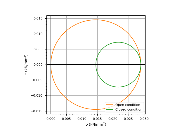
To cause yield in the aluminum, the Von Mises stress would have to exceed the yield strength of the material. For principal stresses \sigma_h and \sigma_l, the Von Mises stress is
\sigma_{eq} = \sqrt{\sigma_h^2 - \sigma_h \sigma_l + \sigma_l^2} \tag{16}
Using Equation 10 and Equation 11, Equation 16 can be rewritten in terms of pressure p, mean radius r, and vessel thickness t.
\begin{aligned} \sigma_{eq} &= \sqrt{\left( \frac{pr}{t} \right)^2 - \left( \frac{pr}{t} \right)\left( \frac{pr}{2t} \right) + \left( \frac{pr}{2t} \right)^2} \\ &= \frac{pr}{t}\sqrt{\frac{3}{4}} \end{aligned} \tag{17}
The yield strength of aluminum is 270~\mathrm{kN/mm^2}. Setting the Von Mises stress equal to the yield strength and solving for pressure, the cylinder is found to yield at 21~\mathrm{kN/mm^2}, or 210000 bar.
4.1 Results
| Gauge | Orientation | Open Reading/ \mu \epsilon | Closed Reading/ \mu \epsilon |
|---|---|---|---|
| G1 | 0° (Longitudinal) | -83.325 | 64.354 |
| G2 | 30° | 36.665 | 130.324 |
| G3 | 45° | 132.102 | 181.066 |
| G4 | 60° | 255.089 | 250.646 |
| G5 | 90° (Hoop) | 360.623 | 309.778 |
4.2 Discussion
Out of all four experiments conducted, the experimental results in the pressure vessel are the worst match for predicted values. The predicted strains overshot the measured strains by 10% or more in all cases. Especially egregious was the longitudinal strain in the “Open” configuration, where the predicted value was off by a factor of nearly 50%! The likeliest explanation for this particular discrepancy is that some longitudinal stress was still expressed in the aluminum cylinder, even in the open position. The negative strain predicted in the “Open” configuration is the lateral contraction resulting from the hoop stress, according to Poisson’s ratio. Any longitudinal stress in the pressure vessel will have the opposite sense and thus counteract that contractive strain.
Jasper Day 2022. Typeset in , with diagrams made in TikZ and the structural analysis library. With thanks to Quarto