Annunciator Project Lab Report
In this report, we create a python program that reads a sparse sensor output, denoises it, and creates various outputs based on that data. The values are plotted live with matplotlib, and an LED light (the “blinkstick”) is illuminated when the values pass user-defined critical amounts.
The Smoothing Algorithm
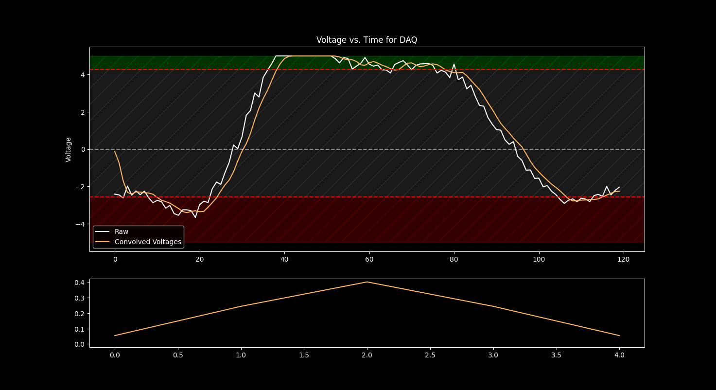
The values read by the sensor contain noise. This noise must be smoothed to prevent flickering of the blinkstick; without smoothing, the variance in the readings would create errors in our estimation of the state of the system. To smooth the noise, the reading is convolved with a gaussian kernel, essentially taking a weighted average around the most recent readings. The gaussian kernel itself is plotted in the lower half of the graph output.
From readings taken at a constant value, a gaussian kernel with size 5 and standard deviation 1 is adequate to reduce the RMS error in the sensor readings by a factor of 50%, which is adequate for the assignment.
Different kernels may be used to yield different results. For a more sensitive reading, the size or deviation of the kernel may be diminished. To make the output less sensitive to veviation and noise, the size or deviation of the kernel may be increased. These settings are changed by altering the KERNEL_SIZE and KERNEL_STANDARD_DEVIATION values at the start of the program. Alternatively, a user-defined kernel may be selected by setting a value for USER_DEFINED_KERNEL.
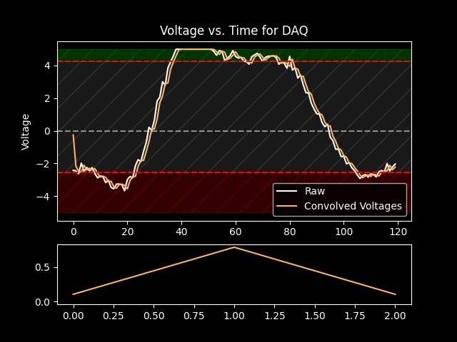
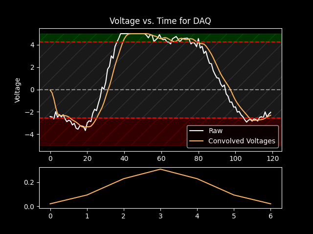
Some different kernels and their effects on the smoothing algorithm are presented Appendix 1.
From Figure 2, the smaller kernel is more sensitive to minor deviations in the readings, and from Figure 3 the larger kernel is less sensitive. The larger kernel is a better choice to increase the confidence in the readings, but it also creates a greater lag between a change in the reading of the sensor and a change in the smoothed values.
Graphing the output
The output from the sensors is graphed live with the matplotlib library. When the Annunciator class is initialized, it is passed artists generated from matplotlib.pyplot.subplots(). All of the graphing then occurs in the Annunciator.update function, which calls various graphing functions elsewhere in the Annunciator class.
The Annunciator class is initialized and then passed to matplotlib's Funcanimation method, which provides the control loop that allows continuous reading and plotting of the sensor output. Every 50 milliseconds (user-definable by the DELTA_T constant), the FuncAnimation method attempts to call annunciator.read_voltage, which obtains the voltage from the sensor. As long as the DELTA_T is set to a duration less than the sampling rate of the sensor, no readings will be dropped by this sampling regime. The read_voltage function itself simply yields the value 1, but when a reading is successfully taken, the data stored in annunciator is mutated.
Blinkstick output
The blinkstick output for the annunciator is much simpler than for the traffic light. Three functions are described which clear the blinkstick, set it to white, and set it to green. The appropriate function is called according to the current value in annunciator.smoothed_voltages as part of the update function.
The code to interface directly with the blinkstick is split off into the BlinkstickAPI function, which provides methods to set the color of the blinkstick to red, green, or clear, as appropriate.
Engineering Applications
Sensors are useful in various engineering applications. In the author’s field of Mechanical Engineering, sensors are used in strain gauges, tachometers, speed readings, vibration readings, and position readings (from cars, boats, robots and rocket ships). All of these sensors create noisy outputs that must be de-noised before they can be used to estimate the state of complex systems. This project demonstrates that step, as well as methods of providing read-outs of sensor data with graphs and LED lights.
Once sensor data has been acquired, it can be used in applications beyond the scope of this project. Several sensors can be combined into a Kalman filter, using knowledge about the system along with multiple live sensor readings to produce more accurate state estimates. But getting denoised data is a good start.
Appendix 1: Graphs and Figures


Appendix 2: Python Code
"""
+============+==========================+
|  Title     |  Annunciator  Project    |
+------------+--------------------------+
|  Author    |  Jasper Day              |
+------------+--------------------------+
|  Date      |  2022.11.17              |
+============+==========================+

This code implements an annunciator panel for a voltage sensor.

The sensor yields a reading corresponding to a voltage between REF_LOW and
    REF_HIGH. The reading is an integer between 0 and 2^BITS. The readings are
    taken every half-second and are plotted live with `matplotlib`.

The voltage readings are smoothed by convolution with a user-defined kernel.
    The Annunciator class gives a method for creating arbitrary Gaussian
    kernels with a given length and standard deviation, or a custom kernel may
    be used.

"""

from scada import DAQ
import matplotlib.pyplot as plt
import matplotlib.animation as animation
from matplotlib import style
import numpy as np
import pandas as pd
from blinkstick import blinkstick

REF_HIGH = +5.0  # high voltage limit on sensor
REF_LOW = -5.0  # low voltage limit on sensor
BITS = 10  # number of bits used to encode the signal
V_HIGH = 4.27  # highest permissible voltage
V_LOW = -2.56  # lowest permissible voltage
KERNEL_SIZE = 7 # size of the convolution kernel for voltage smoothing
KERNEL_STANDARD_DEVIATION = 1.3 # standard deviation of the convolution kernel
USER_DEFINED_KERNEL = False # change to list of values for custom kernel
DELTA_T = 50 # Milliseconds between sensor reading attempts


style.use("dark_background")

# Data Acquisition setup

my_daq = DAQ(matric="s2265891", user="Jasper Day")
my_daq.connect("coursework")
my_daq.trigger()

class BlinkstickAPI():
    # interface to easily change blinkstick
    def __init__(self):
        self.bstick = blinkstick.find_first()
        if self.bstick == None:
            raise Exception("No blinkstick found")

    def clear_colors(self):
        for led in range(0,8):
            self.bstick.set_color(index=led, name="black")

    def set_red(self):
        for led in range(0,8):
            self.bstick.set_color(index=led, name="red")

    def set_green(self):
        for led in range(0,8):
            self.bstick.set_color(index=led, name="green")


# The Annunciator class implements a digital display of the current voltage
# readout, as well as interfacing with the blinkstick.

class Annunciator:
    def __init__(self, axs, daq):
        self.ax = axs[0]
        self.axkernel = axs[1]
        self.daq = daq
        # Data structure
        self.voltages = []
        self.array_length = 120
        self.convolved_voltages = []
        # Blinkstick
        try:
            self.blinkstick = BlinkstickAPI()
        except:
            print("No blinkstick found.")
        # Set kernel
        if not USER_DEFINED_KERNEL:
            self.kernel = self.gaussian_kernel(length=KERNEL_SIZE, sigma=KERNEL_STANDARD_DEVIATION)
        else:
            self.kernel = USER_DEFINED_KERNEL
        self.kernel_length = len(self.kernel)

    def update(self, frame):

        # smooth readings
        self.convolve_voltage()

        # update blinkstick
        self.update_blinkstick()

        # plot results
        self.plot_setup()
        self.plot_voltages()
        self.plot_voltage_limits()
        self.plot_kernel()

        print("# of voltage readings: " + str(len(self.voltages)))
        print("Length of convolved vector: " + str(len(self.convolved_voltages)))

    def read_voltage(self):
        cur_time, cur_volts = self.daq.next_reading()
        # Reverse-engineering voltage from 10 bit reading
        Q = (REF_HIGH - REF_LOW) / 2**BITS
        cur_volts_converted = cur_volts * Q + REF_LOW
        # print output to terminal
        print(
            "The time is "
            + str(cur_time)
            + " and the voltage is "
            + str(cur_volts_converted)
        )
        self.voltages.append(cur_volts_converted)
        yield 1

    def gaussian_kernel(self, length=5, sigma=0.8):
        # Create even / odd kernel centered around 0
        if length % 2 == 0:
            kernel = np.linspace(-length / 2, length / 2 - 1, length)
        else:
            kernel = np.linspace(-(length - 1) / 2.0, (length - 1) / 2.0, length)

        # gaussian = e ^ (-0.5 x^2/σ^2)
        kernel = np.exp(-0.5 * np.square(kernel) / np.square(sigma))

        # normalize kernel
        return kernel / np.sum(kernel)

    def convolve_voltage(self):
        self.convolved_voltages = np.convolve(self.voltages, self.kernel)[0:-self.kernel_length + 1]

    def update_blinkstick(self):
        # check most recent smoothed reading
        if self.convolved_voltages[-1] < V_LOW:
            self.blinkstick.set_red()
        elif self.convolved_voltages[-1] > V_HIGH:
            self.blinkstick.set_green()
        else:
            self.blinkstick.clear_colors()

    def plot_setup(self):
        # Clear all axes
        self.ax.clear()
        self.axkernel.clear()
        # Title and labels
        self.ax.set_title("Voltage vs. Time for DAQ")
        self.ax.set_ylabel("Voltage")
        # Ylimits
        self.ax.set_ylim(REF_LOW - 0.5, REF_HIGH + 0.5)

    def plot_voltage_limits(self):
        # Graph upper and lower limits for voltage
        self.ax.axhline(y=V_LOW, color="red", linestyle="--")
        self.ax.axhline(y=V_HIGH, color="red", linestyle="--")
        self.ax.axhline(y=0, color="w", linestyle="--", alpha=0.5)
        self.ax.fill_between(
            x=self.ax.set_xlim(), y1=V_LOW, y2=V_HIGH, color="w", hatch="/", alpha=0.1
        )
        self.ax.fill_between(
            x=self.ax.set_xlim(), y1=REF_LOW, y2=V_LOW, color="r", hatch="/", alpha=0.2
        )
        self.ax.fill_between(
            x=self.ax.set_xlim(), y1=V_HIGH, y2=REF_HIGH, color="g", hatch="/", alpha=0.4
        )

    def plot_voltages(self):
        # Raw (measured) voltages
        self.ax.plot(self.voltages, color="w", label="Raw")
        # Convolved (smoothed) voltages
        self.ax.plot(self.convolved_voltages, color="C5", label="Convolved Voltages")
        self.ax.legend()

    def plot_kernel(self):
        self.axkernel.axhline(y=0, linestyle="--", color="black", alpha=0.5)
        self.axkernel.plot(self.kernel, color="C5", label="kernel")
        # Fancy lights
        if self.convolved_voltages[-1] < V_LOW:
            self.axkernel.fill_between(
                x=(
                    self.axkernel.get_xlim()[0] + 0.5,
                    self.axkernel.get_xlim()[1] - 0.5,
                ),
                y1=0,
                y2=np.amax(self.kernel),
                color="red",
                alpha=0.2,
            )
        if self.convolved_voltages[-1] > V_HIGH:
            self.axkernel.fill_between(
                x=(
                    self.axkernel.get_xlim()[0] + 0.5,
                    self.axkernel.get_xlim()[1] - 0.5,
                ),
                y1=0,
                y2=np.amax(self.kernel),
                color="green",
                alpha=0.4,
            )

# CONTROL FLOW STARTS HERE

fig, axs = plt.subplots(2, gridspec_kw={"height_ratios": [3, 1]})

annunciator = Annunciator(axs, my_daq)

ani = animation.FuncAnimation(
    fig, annunciator.update, annunciator.read_voltage, interval=DELTA_T
)

plt.show()